This post will be a high-level overview of the main ideas behind the paper, Generative Modeling via Drifting.

Setup

Generative modelling can be formulated as learning a function $f$ that maps a known prior distribution $p_{\text{prior}}$ to a target distribution (usually the data itself) $p_{\text{data}}$.

Let's assume that the prior distribution is a standard Gaussian (standard in the generative models) and the target distribution is the data distribution. Since training a neural network via gradient descent is inherently an iterative process, it's reasonable to assume that during training, we'd have access to a function $f_i$ that maps $p_{\epsilon}$ to $q_i$, which is our approximation to $p_{\text{data}}$ at iteration $i$. So, for each iteration, there is a "drift" between a sample at the $i$-th iteration and that at the $(i + 1)$-th iteration. We can write:

where $\Delta_i = f_{i + 1}(\epsilon) - f_i(\epsilon)$

If $\Delta_i = 0$, we have reached an equilibrium point where it doesn't make sense to continue training.

Let's make this more formal. The authors introduce the notion of a drfiting field $V_{p, q}$ as a way to model $\Delta_i$, so

where $x_i = f_i(\epsilon)$ and $\epsilon \sim p$, and $x_i \sim q_i$. When $p = q$, we want the drifting field $V_{p, q}$ to be 0. This notion of equilibrium motivates an update rule:

Here $\theta_i$ are the parameters of the model at iteration $i$. The loss function is the mean-squared error of $x_{i + 1}$ and $x_i$:

We use a stopgrad since we want to freeze our target and move our current predicted samples towards it.

Designing the Drifting Field

Now how should we design $V$? Recall that we wish to find our In the paper, they give a sufficient (but not necessary) condition: make $V$ anti-symmetric. To see this, note that $p = q \implies V_{p, q} = -V_{q, p} = -V_{p, q} = 0$.

The paper considers drifting fields of the form:

where $\mathcal{K}$ is a function describing interactions on sampled points from the target distribution and the current estimate of it. Here $\mathcal{K}$ just needs to be 0 when $p = q$.

The authors define fields

and decompose $V_{p, q}(x)$ into a difference $V_p^+(x) - V_q^-(x)$. Here $Z_p$ and $Z_q$ are normalization constants $\mathbb{E}_p[k(x, y^+)]$ and $\mathbb{E}_q[k(x, y^-)]$, respectively. We can rewrite $V_{p, q}(x)$ as follows:

The reason we can rewrite terms $E_p[f(y^+)]$, $E_q[g(y^-)]$ into a combined expression $E_{p, q}[f(y^+)g(y^-)]$ is because the variables $y^+\sim p$, $y^-\sim q$ are drawn separately, so their product can be written as an expectation over the product measure $p \times q$.

From this, it's immediately obvious that $V_{p, q}$ is anti-symmetric, so our training objective discussed earlier is well-defined. The kernel $k$ they used was

Implementation Details

We give a concrete implementation of the drifting field above:

def compute_drift_field(x_bd, ypos_bd, yneg_bd, temp: float = 0.05, eps: float = 1e-12):
    """
    Computes the drift field V_pq(f(eps))
    
    :param x_bd: [N, D]
    :param ypos_bd: p, distribution of the data. [N_pos, D]
    :param yneg_bd: q, current distribution. [N_neg, D]
 
    Note that the batch dimensions of the data and generated predictions
    do not have to be the same.
 
    Returns a [N, D] matrix representing a drift field.
    """
 
    targets = jnp.concatenate([yneg_bd, ypos_bd], axis=0)
    N_neg = x_bd.shape[0]
 
    dist = cdist(x_bd, targets)
    # since x_bd is the same as yneg_bd, mask self
    dist = dist.at[:, :N_neg].add(jnp.eye(N_neg) * 1e6)
    kernel = jnp.exp(-dist / temp)
 
    normalizer = jnp.sum(kernel, axis=-1, keepdims=True) * jnp.sum(kernel, axis=-2, keepdims=True)
    normalizer = jnp.sqrt(jnp.clip(normalizer, a_min=eps))
    normalized_kernel = kernel / normalizer
 
    K_neg, K_pos = jnp.split(normalized_kernel, [N_neg,], axis=1)
 
    pos_coeff = K_pos * jnp.sum(K_neg, axis=-1, keepdims=True)
    V_pos = pos_coeff @ ypos_bd
    neg_coeff = K_neg * jnp.sum(K_pos, axis=-1, keepdims=True)
    V_neg = neg_coeff @ yneg_bd
 
    return V_pos - V_neg

To see how this can be written in the form $\frac{1}{Z_pZ_q}\mathbb{E}_{p, q}[k(x, y^+)k(x, y^-)(y^+ - y^-)]$, observe that $V_p^+(x) = \sum_{i}\alpha_i^+\left(\sum_j\alpha_j^-\right)y^+$ and $V_q^-(x) = \sum_{i}\alpha_j^-\left(\sum_i\alpha_i^+\right)y^-$

Combining the two, we get that

which is exactly the form that we wanted. Here it's clear that $\alpha_i^+$ and $\alpha_i^-$ represent $k(x, y^+)$ and $k(x, y^-)$ respectively.

What about the normalization terms $Z_p$ and $Z_q$. When we compute $k$, we bake in the normalization by summing across the concatenated $y = [y^+; y^-]$ dimension and dividing by that constant. We also normalize over the batch dimension as it improved training dynamics.

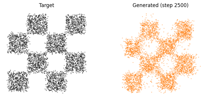
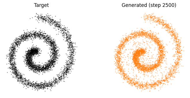
Experiments on Toy Distributions

A JAX implementation of the above can be found here:

I was able to train the model on the toy distributions (chessboard, spiral). After 2.5k iterations, the drifting model produced some pretty neat results.

Extending this to Actual Large-Scale Image Datasets

Much like other work such as Diffusion Transformers, this method can work on encoded features instead of raw pixels. Let $\phi$ be a feature encoder. We can define our new loss as:

where $\phi(x) = f_{\theta}(\epsilon)$. The update rule is changed similarly.