Graph based representations of molecules have been an active area of research in recent years, with downstream applications in property prediction (HOMO-LUMO gap and various energy properties), to generative modeling of the molecules itself.

We'll explore the generative modelling aspect. It's no secret that genrative models (GenAI in popular lexicon) has taken the world by storm in recent years. There has been remarkable progress in image, text, and video generation. And with some additional effort, generating higher representations of the above (such as code and mathematical proofs) have also seen amazing progress.

One (admittedly outdated by now) method of generative models is score models. This post aims to explain what they are and how they have been applied to the task of generating accurate of molecules as a 3D coordinate matrices. In the ML literature, this task is usually referred to as conformer prediction.

Score Models

Suppose we have a dataset $\{x_1, ..., x_N\}$. Instead of training to maximize the log-likelihood of the data:

$$\text{max}_{\theta} \sum_{i = 1}^N p_{\theta}(x)$$

by modelling $p_{\theta}$ directly, score models try to learn a model $s_{\theta}$ that approximates $\nabla_x \text{log }p_{\text{data}}(x)$. The training objective for score models amounts to minimizing the following objective function:

$$\mathbb{E}_{p_{\text{data}}} \left[ \left\lVert s_{\theta}(x) - \nabla_x \text{log }p_{\text{data}}(x)\right\rVert_2^2 \right]$$

This objective function can be shown to be equivalent to the minimizing the following:

$$\mathbb{E}_{p_{\text{data}}} \left[ \text{Tr}(\nabla_x s_{\theta}(x)) + \frac{1}{2}\left\lVert s_{\theta}\right\rVert_2^2 \right]$$

The trace term is computationally prohibitive, and there have been there are some works to approximate it. One approach, called denoising score matching, is when we perturb a data point x via a predefined noise distribution $q_{\sigma}(\tilde{x} | x)$ and estimate the score of the perturbed data distribution $q_{\sigma}(\tilde{x})$. The objective to be minimized is now the following:

$$\frac{1}{2}\mathbb{E}_{q_{\sigma}(\tilde{x} | x)} \mathbb{E}_{p_{\text{data}}} \left[ \left\lVert s_{\theta}(\tilde{x}) - \nabla_{\tilde{x}} \text{log }q_{\sigma}(\tilde{x} | x) \right\rVert_2^2 \right]$$

In the paper Generative Modeling by Estimating Gradients of the Data Distribution, Song et al. sets $q_{\sigma}(\tilde{x} | x)$ as a Gaussian with mean $x$ and covariance $\sigma^2I$. The score model takes in an additional parameter $s_{\theta}(x, \sigma)$, hence the name Noise Conditional Score Network.

Since $\nabla_{\tilde{x}} \text{log }q_{\sigma}(\tilde{x} | x) = -\frac{\tilde{x} - x}{\sigma^2}$, the loss objective can be simplified to:

$$\frac{1}{2}\mathbb{E}_{q_{\sigma}(\tilde{x} | x)} \mathbb{E}_{p_{\text{data}}} \left[ \left\lVert s_{\theta}(\tilde{x}) + \frac{\tilde{x} - x}{\sigma^2} \right\rVert_2^2 \right]$$

In practice, we use Monte-Carlo estimation to compute the expectation across $\mathbb{E}_{p_{\text{data}}}$ and $\mathbb{E}_{q_{\sigma}}$.

Sampling from a Score Model

Now that we have a trained score-model, how do we actually sample data? Langevin dynamics states that the following formula:

$$x_t = x_{t - 1} + \frac{\epsilon}{2}s_{\theta}(x)+ \sqrt{\epsilon}z_t$$

where $z_t \sim \mathcal{N}(0, I)$ ensure that $x_t$ will match the data distribution as $t$ goes to infinity. In the NCSN framework, we follow an annealed version of this:

$$x_t = x_{t -1} + \frac{\epsilon}{2} \cdot \frac{\sigma_i}{\sigma_L}s_{\theta}(x, \sigma_i) + \sqrt{\epsilon}z_t$$

Applying Score Models to Molecular Conformation

Shi et al. were able to apply NCSN's to molecular conformation in Learning Gradient Fields for Molecular Conformation Generation. Let's revisit the conformation generation setup. We can represent a molecule as a graph $G = (V, E)$, where each $v_i \in V$ is an atom with various node features (atomic number, charge), and each $e_{ij} \in E$ represents a bond between atoms $i$ and $j$. Each edge also has it's own features such as bond type and distance. Our task is given a graph $G$, predict a 3D coordinate matrix $R \in \mathbb{R}^{|V| \times 3}$.

Conceptually, what we want is to train a score model that estimates $\nabla_R \text{log }(R | G)$. This score model needs to be invariant to translation (shifting coordinates by a constant should yield ths same score), and equivariant to rotations (the gradient should rotate along with the coordinates).

In the paper, they make a pretty clever modelling choice. Instead of training a score model directly on a conformation $R$, they train a score model on the interatomic distances. This method still works because interatomic distances are invariant to rotation and translation. Therefore, standard graph neural networks can be used while implicitly enforcing intrinsitc geometry, since generating accurate distances implicitly enforces certain geometric constraints. The authors also use 2/3-hop neighbors in the edge matrix $E$ to enfore even more geometric constraints.

But given a score model for interatomic distances, $d_ij$, how do we compute the score for a conformer? By breaking down $\nabla_R \text{log }(R | G) = f_G(d) \circ g(R)$, where $g$ is a function that computes the interatomic distances and $f_G$ is a GNN taking the molecule features and a distance vector and outputs a conformation or a molecule-level property.

Luckily, these two quantities are related by the chain rule:

$$s_{\theta}(R)_i = \frac{\partial f_G(d)}{\partial r_i} = \sum_{e_{ij} \in E} \frac{\partial f_G(d)}{\partial d_{ij}} \cdot \frac{\partial d_{ij}}{\partial r_i} = \sum_{e_{ij} \in E} s_{\theta}(d)_{ij} \cdot \frac{1}{d_{ij}} \left\lVert r_i - r_j \right\rVert$$

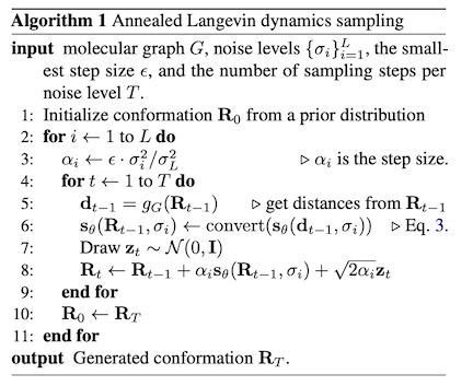
During sampling, we operate on the distances, and use the chain rule to convert our learned score model over distances to a score model over the respective conformer $s_{\theta}(R)_i$. The sampling pseudocode is outlined below:

On the conformation prediction task, it achieved SOTA results (for the time).

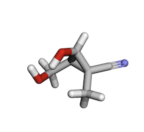
I was able to implement this in JAX. And here is an example of a sample I was able to generate.

Take a look at my implementation of this paper here.